Visually communicate your scientific data with R

Designing scientific figures

Eric Largy

eric.largy@u-bordeaux.fr

ARNA, INSERM U1212, CNRS UMR 5320, Université de Bordeaux

UFR des Sciences Pharmaceutiques, Université de Bordeaux

April 22, 2026

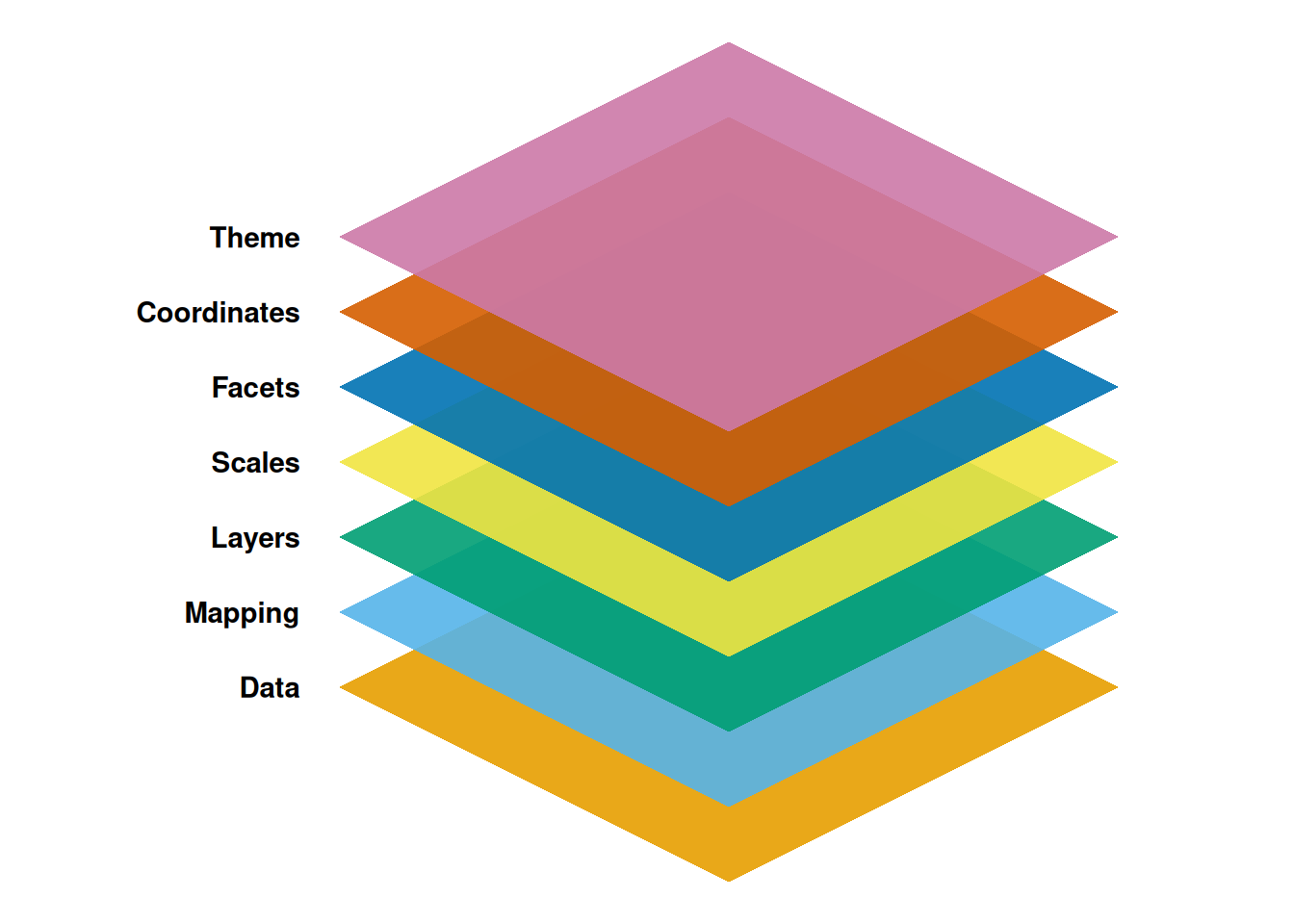
Introduction to Grammar of Graphics

A framework for data visualization

Introduced by Leland Wilkinson (The Grammar of Graphics, 2005).

Graphics can be built up from a set of components:

Data: the dataset to be visualized
Variables: mapping of objects to values
Algebra: operations to combine variables and specify dimensions
Scales: represent variables on measured dimensions
Statistics: functions to change the appearance and representation

Geometry: creation of geometric graphs from variables
Coordinates: mapping to coordinate systems
Aesthetics: sensory attributes
Facets: subplots based on subsets of data
Guides: legends and axes to explain the graph

Adapted to R in the `ggplot2` package

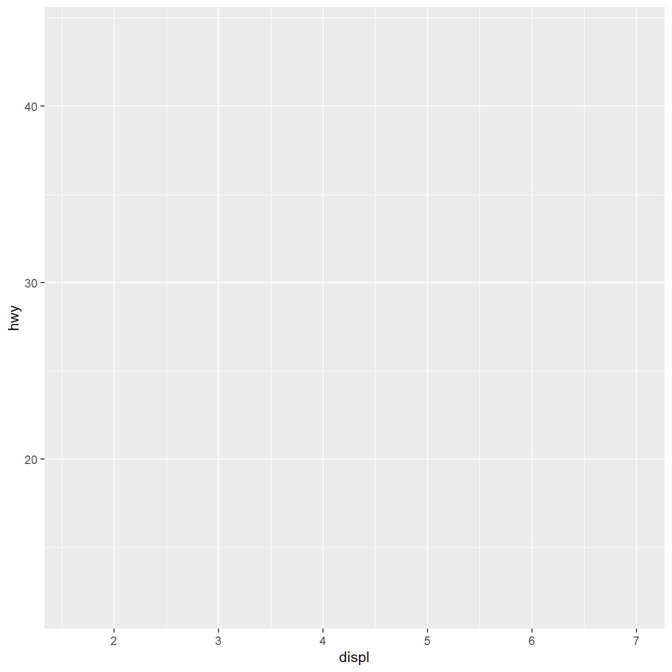
Example: Data should be formatted with 1 column per variable

library(dplyr)
library(data.table)
library(DT)
library(ggplot2)

DT::datatable(mpg)

ggplot initialization provides a plotting area

library(ggplot2)

ggplot(mpg)

Mapping x and y coordinates provide axes

library(ggplot2)

ggplot(
  mpg,
  mapping = aes(x = displ, y = hwy)
)

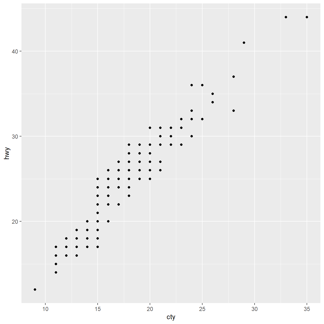
Geometries can be added as layers

library(ggplot2)

ggplot(
  mpg,
  mapping = aes(
    x = cty,
    y = hwy
  )
) +
  geom_point()

Scales can be applied to aesthetics

library(ggplot2)

ggplot(
  mpg,
  mapping = aes(
    x = displ,
    y = hwy,
    colour = class
  )
) +
  geom_point() +
  scale_colour_viridis_d()

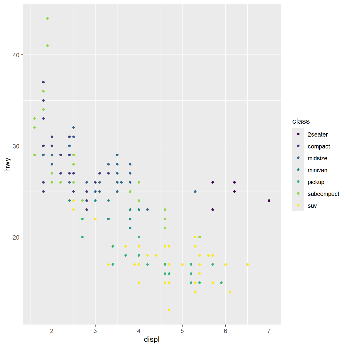
Facetting allows generating many subplots

library(ggplot2)

ggplot(
  mpg,
  mapping = aes(
    x = displ,
    y = hwy,
    colour = class
  )
) +
  geom_point() +
  scale_colour_viridis_d() +
  facet_grid(year ~ class)

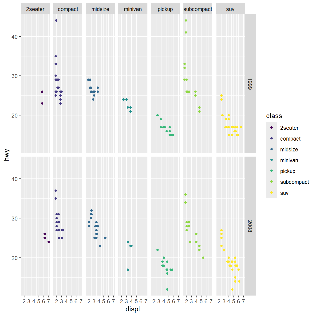
Coordinates allows re-scaling

library(ggplot2)

ggplot(
  mpg,
  mapping = aes(
    x = displ,
    y = hwy,
    colour = class
  )
) +
  geom_point() +
  scale_colour_viridis_d() +
  facet_grid(year ~ class) +
  coord_cartesian(
    xlim = c(0, 8),
    ylim = c(10, 50)
  )

Make it pretty/corporate/legible with a theme

library(ggplot2)

ggplot(
  mpg,
  mapping = aes(
    x = displ,
    y = hwy,
    colour = class
  )
) +
  geom_point() +
  scale_colour_viridis_d() +
  facet_grid(year ~ class) +
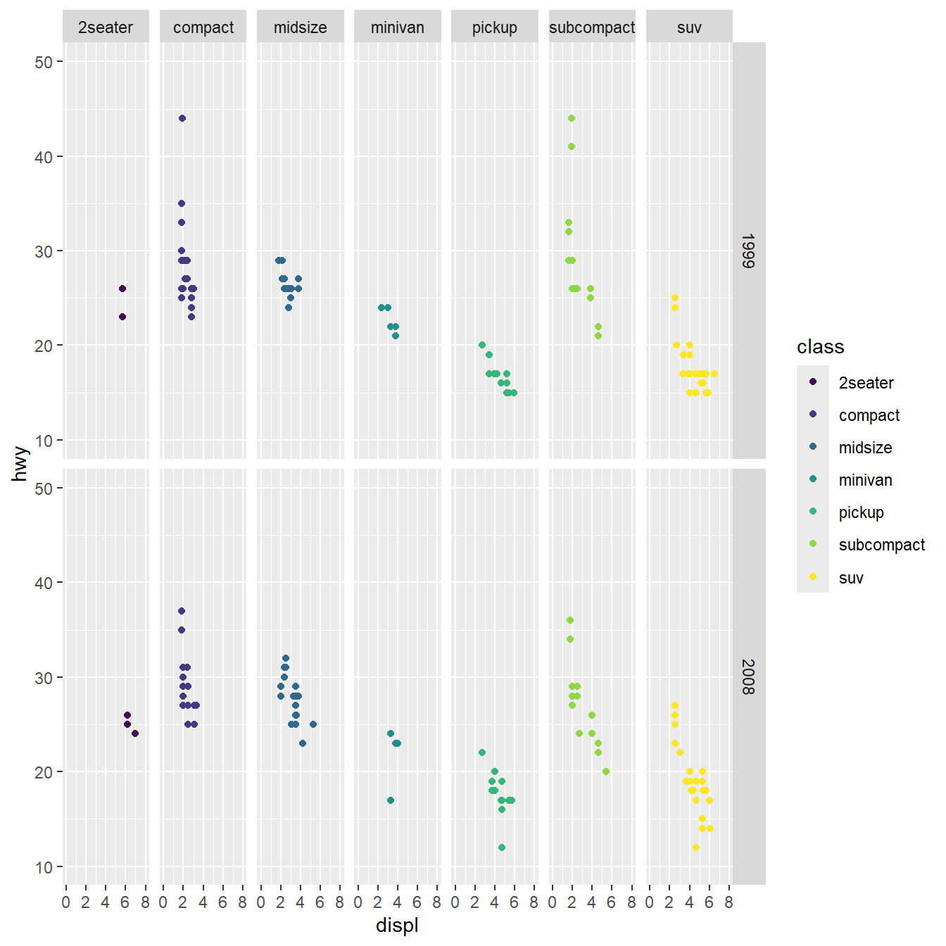
  coord_cartesian(
    xlim = c(0, 8),
    ylim = c(10, 50),
    clip = "off"
  ) +
  theme_minimal() +
  theme(
    panel.grid.major = element_blank(),
    panel.grid.minor = element_blank(),
    legend.position = "bottom",
    axis.title = element_text(size = 14, face = "bold"),
    axis.line = element_line(color = "black", size = 0.75),
    axis.ticks = element_line(color = "black", size = 0.75),
    legend.title = element_text(face = "bold", size = 10),
    legend.text = element_text(size = 10),
    strip.text = element_text(face = "bold", size = 10)
  ) +
  scale_x_continuous(
    name = "Engine Displacement (L)",
    breaks = seq(0, 8, 4),
    limits = c(0, 8),
    expand = c(0, 0)
  ) +
  scale_y_continuous(name = "Highway Miles per Gallon") +
  labs(colour = "Vehicle Class")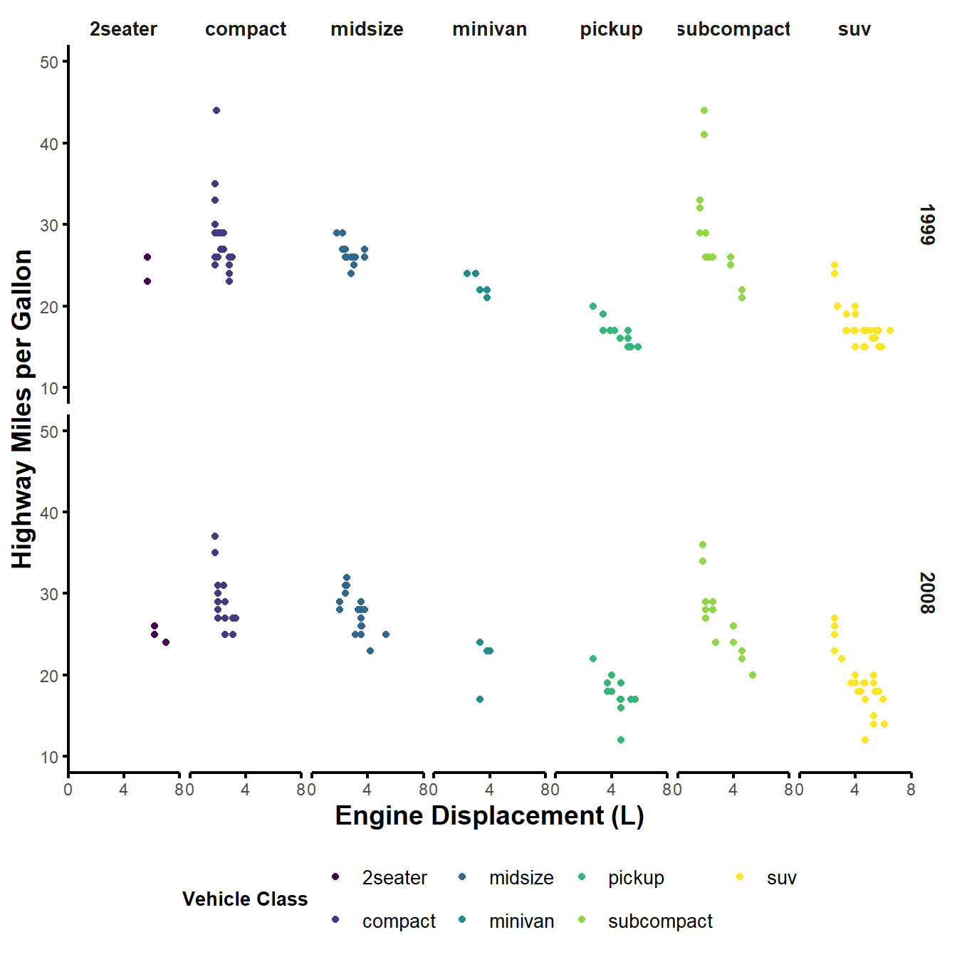

Setup of the environment

Tidyverse install verification

if (!requireNamespace("tidyverse", quietly = TRUE)) {
  install.packages("tidyverse")
}

library(tidyverse)

Data.table install verification

if (!requireNamespace("data.table", quietly = TRUE)) {
  install.packages("data.table")
}

library(data.table)

# version check
packageVersion("data.table")

[1] '1.17.99'

Reminders on variables and data types and modes

Assigning and printing numeric variables

a <- 42L
b <- 42
c <- pi

print(a) # prints the value of a

[1] 42

a # also prints the value of a

[1] 42

class(a) # integer is a class

[1] "integer"

# integer is a type
# (32-bit integer storage)
typeof(a)

[1] "integer"

class(b) # numeric is a class

[1] "numeric"

# numeric type stored as double
# (64-bit floating point)
typeof(b)

[1] "double"

class(c)

[1] "numeric"

typeof(c)

[1] "double"

Assigning and printing character variables

a_string <- "fourty-two"

a_string

[1] "fourty-two"

Assigning and printing boolean variables

a_boolean <- TRUE
b_boolean <- FALSE

c(a_boolean, b_boolean)

[1]  TRUE FALSE

Null, missing values and infinities

a_null <- NULL
a_missing <- NA
a_nan <- NaN
a_inf <- Inf
a_minus_inf <- -Inf
char_missing <- NA_character_
real_missing <- NA_real_
int_missing <- NA_integer_

str(
  list(
    a_null = a_null,
    a_missing = a_missing,
    a_nan = a_nan,
    a_inf = a_inf,
    a_minus_inf = a_minus_inf,
    char_missing = char_missing,
    real_missing = real_missing,
    int_missing = int_missing
  )
)

List of 8
 $ a_null      : NULL
 $ a_missing   : logi NA
 $ a_nan       : num NaN
 $ a_inf       : num Inf
 $ a_minus_inf : num -Inf
 $ char_missing: chr NA
 $ real_missing: num NA
 $ int_missing : int NA

A NULL value is not missing

a_null <- NULL
a_missing <- NA
a_nan <- NaN
a_inf <- Inf
a_minus_inf <- -Inf
char_missing <- NA_character_
real_missing <- NA_real_
int_missing <- NA_integer_

cat(
  "NULL represents the absence of a value or object,",
  "\nwhile NA represents a missing value in a vector.",
  "\n\nThe length of a NULL value is",
  length(a_null),
  ",\nwhile the length of a missing value is",
  length(a_missing),
  "."
)

NULL represents the absence of a value or object, 
while NA represents a missing value in a vector. 

The length of a NULL value is 0 ,
while the length of a missing value is 1 .

Factors are important for ordering elements in visualizations

a_factor <- factor(
  c("low", "medium", "high", "medium", "low")
)

a_factor

[1] low    medium high   medium low   
Levels: high low medium

# Removing the "medium" level from the factor
droplevels(a_factor, "medium")

[1] low  <NA> high <NA> low 
Levels: high low

# Adding data with a new level "very high"
new_data <- c("very high", "low")
factor_vec <- c(
  a_factor,
  factor(new_data, levels = c(levels(a_factor), "very high"))
)
factor_vec

[1] low       medium    high      medium    low       very high low      
Levels: high low medium very high

Creating vectors

# Explicit creation
a_vector <- c(1:10, "coucou")

a_vector

 [1] "1"      "2"      "3"      "4"      "5"      "6"      "7"      "8"     
 [9] "9"      "10"     "coucou"

# Implicit integer creation
int_vector <- 1:10

int_vector

 [1]  1  2  3  4  5  6  7  8  9 10

R coerces all elements to the most flexible type

a_vector <- c(1:10, "coucou")

class(a_vector)

[1] "character"

Subsetting vectors by position, logical and negative indexing

a_vector <- c(1:10, "coucou")
# R is 1-indexed
# so the first element is at position 1
a_vector[c(1:3, 11)]

[1] "1"      "2"      "3"      "coucou"

# Logical indexing
a_vector[
  c(TRUE, TRUE, TRUE, rep(FALSE, 7), TRUE)
]

[1] "1"      "2"      "3"      "coucou"

# Negative indexing
a_vector[-c(4:10)]

[1] "1"      "2"      "3"      "coucou"

Naming vector elements

b_vector <- c(1:5)

names(b_vector) <- c(
  "one",
  "two",
  "three",
  "four",
  "five"
)

b_vector

  one   two three  four  five 
    1     2     3     4     5

Accessing named vector elements with `[]` and `[[]]`

b_vector["three"] #named element

three 
    3

b_vector[["three"]] #scalar element

[1] 3

Modifying elements and types of a vector

b_vector <- c(1:5)

a <- 42

b_vector[3] <- a

b_vector[1] <- "one"

b_vector

[1] "one" "2"   "42"  "4"   "5"

b_vector[1] <- 1

b_vector

[1] "1"  "2"  "42" "4"  "5"

# Coercion to integer
# Only for printing here!
# The original vector is still character!
as.integer(b_vector)

[1]  1  2 42  4  5

Creating and inspecting lists

# lists cannot contain
# different types of data
# but can contain different types of objects,
# including vectors

a_list <- list(
  numeric_vector = c(1, 2, 3, 4),
  character_vector = c("a", "b", "c"),
  mixed_vector = c(1, "b", TRUE),
  nested_list = list(
    numeric_vector = c(5, 6, 7, 8),
    character_vector = c("d", "e", "f"),
    mixed_vector = c(9, "g", FALSE)
  )
)

a_list

$numeric_vector
[1] 1 2 3 4

$character_vector
[1] "a" "b" "c"

$mixed_vector
[1] "1"    "b"    "TRUE"

$nested_list
$nested_list$numeric_vector
[1] 5 6 7 8

$nested_list$character_vector
[1] "d" "e" "f"

$nested_list$mixed_vector
[1] "9"     "g"     "FALSE"

Accessing list elements by name with `$`

a_list <- list(
  numeric_vector = c(1, 2, 3, 4),
  character_vector = c("a", "b", "c"),
  mixed_vector = c(1, "b", TRUE),
  nested_list = list(
    numeric_vector = c(5, 6, 7, 8),
    character_vector = c("d", "e", "f"),
    mixed_vector = c(9, "g", FALSE)
  )
)

a_list$mixed_vector

[1] "1"    "b"    "TRUE"

Accessing nested list elements by name with `$`

a_list <- list(
  numeric_vector = c(1, 2, 3, 4),
  character_vector = c("a", "b", "c"),
  mixed_vector = c(1, "b", TRUE),
  nested_list = list(
    numeric_vector = c(5, 6, 7, 8),
    character_vector = c("d", "e", "f"),
    mixed_vector = c(9, "g", FALSE)
  )
)

a_list$nested_list$character_vector

[1] "d" "e" "f"

Comparing list elements for equality

a_list <- list(
  numeric_vector = c(1, 2, 3, 4),
  character_vector = c("a", "b", "c"),
  mixed_vector = c(1, "b", TRUE),
  nested_list = list(
    numeric_vector = c(5, 6, 7, 8),
    character_vector = c("d", "e", "f"),
    mixed_vector = c(9, "g", FALSE)
  )
)

all(a_list$nested_list$character_vector == a_list$character_vector)

[1] FALSE

all(a_list$nested_list$character_vector == a_list$character_vector)

[1] FALSE

(a_list$numeric_vector[1] + 4) == a_list$nested_list$numeric_vector[1]

[1] TRUE

Subsetting lists: `[ ]` vs. `[[ ]]`

a_list <- list(
  numeric_vector = c(1, 2, 3, 4),
  character_vector = c("a", "b", "c"),
  mixed_vector = c(1, "b", TRUE),
  nested_list = list(
    numeric_vector = c(5, 6, 7, 8),
    character_vector = c("d", "e", "f"),
    mixed_vector = c(9, "g", FALSE)
  )
)

str(
  list(
    'dollar_name' = a_list$character_vector,
    'bracket_name' = a_list[["character_vector"]],
    'bracket_index' = a_list[[2]],
    'bracket_twice' = a_list[2][[1]]
  )
)

List of 4
 $ dollar_name  : chr [1:3] "a" "b" "c"
 $ bracket_name : chr [1:3] "a" "b" "c"
 $ bracket_index: chr [1:3] "a" "b" "c"
 $ bracket_twice: chr [1:3] "a" "b" "c"

What happens if we access a_list[2] vs. a_list[[2]]?

a_list[2]

$character_vector
[1] "a" "b" "c"

a_list[[2]]

[1] "a" "b" "c"

Creating matrices

mat <- matrix(1:9, nrow = 3)

mat

     [,1] [,2] [,3]
[1,]    1    4    7
[2,]    2    5    8
[3,]    3    6    9

matrix(1:9, nrow = 3)

     [,1] [,2] [,3]
[1,]    1    4    7
[2,]    2    5    8
[3,]    3    6    9

matrix(1:8, nrow = 3)

Warning in matrix(1:8, nrow = 3): data length [8] is not a sub-multiple or
multiple of the number of rows [3]

     [,1] [,2] [,3]
[1,]    1    4    7
[2,]    2    5    8
[3,]    3    6    1

Indexing matrices by row and column

mat <- matrix(1:9, nrow = 3)

mat

     [,1] [,2] [,3]
[1,]    1    4    7
[2,]    2    5    8
[3,]    3    6    9

mat[1, ] # First row

[1] 1 4 7

mat[, 2] # Second column

[1] 4 5 6

mat[1, 2] # Element at row 1, column 2

[1] 4

Creating dataframes as named list of vectors

a_df <- data.frame(
  id = 1:5,
  group = c("A", "A", "B", "B", "C"),
  value = c(10.2, 12.5, 9.8, 11.1, 13.0)
)

a_df

  id group value
1  1     A  10.2
2  2     A  12.5
3  3     B   9.8
4  4     B  11.1
5  5     C  13.0

Accessing column names with `names()`

a_df <- data.frame(
  id = 1:5,
  group = c("A", "A", "B", "B", "C"),
  value = c(10.2, 12.5, 9.8, 11.1, 13.0)
)

names(a_df)

[1] "id"    "group" "value"

Accessing dataframe columns with `$`

a_df <- data.frame(
  id = 1:5,
  group = c("A", "A", "B", "B", "C"),
  value = c(10.2, 12.5, 9.8, 11.1, 13.0)
)

a_df$group

[1] "A" "A" "B" "B" "C"

cat(
  "It is",
  is.vector(a_df$group),
  "that a_df$group is a vector, containing",
  class(a_df$group),
  "data."
)

It is TRUE that a_df$group is a vector, containing character data.

Accessing dataframe columns with `$`

a_df <- data.frame(
  id = 1:5,
  group = c("A", "A", "B", "B", "C"),
  value = c(10.2, 12.5, 9.8, 11.1, 13.0)
)

unique(a_df$group)

[1] "A" "B" "C"

sort(a_df$value)

[1]  9.8 10.2 11.1 12.5 13.0

sort(a_df$value, decreasing = TRUE)

[1] 13.0 12.5 11.1 10.2  9.8

Subsetting dataframes by row/column indices

a_df <- data.frame(
  id = 1:5,
  group = c("A", "A", "B", "B", "C"),
  value = c(10.2, 12.5, 9.8, 11.1, 13.0)
)

# Select rows 1 and 3, all columns
a_df[c(1, 3), ]

  id group value
1  1     A  10.2
3  3     B   9.8

# Select all rows, columns 1 and 3
a_df[, c(1, 3)]

# Select rows 1 to 3, columns "id" and "value"
a_df[1:3, c("id", "value")]

  id value
1  1  10.2
2  2  12.5
3  3   9.8

# Select rows where group is "A" or "B",
# and columns 1 to 3
a_df[
  a_df$group %in% c("A", "B"),
  1:3
]

  id group value
1  1     A  10.2
2  2     A  12.5
3  3     B   9.8
4  4     B  11.1

Subsetting dataframes by column names

a_df <- data.frame(
  id = 1:5,
  group = c("A", "A", "B", "B", "C"),
  value = c(10.2, 12.5, 9.8, 11.1, 13.0)
)

a_df[c("id", "value")]

a_df[["group"]] # access to scalar vector

[1] "A" "A" "B" "B" "C"

Subsetting dataframes by logical conditions

a_df <- data.frame(
  id = 1:5,
  group = c("A", "A", "B", "B", "C"),
  value = c(10.2, 12.5, 9.8, 11.1, 13.0)
)

# Rows where value > 10
a_df[a_df$value > 10, ]

  id group value
1  1     A  10.2
2  2     A  12.5
4  4     B  11.1
5  5     C  13.0

# Rows where group is "A" AND value > 10
a_df[a_df$group == "A" & a_df$value > 10, ]

  id group value
1  1     A  10.2
2  2     A  12.5

Subsetting dataframes can be subsetted with `subset()`

a_df <- data.frame(
  id = 1:5,
  group = c("A", "A", "B", "B", "C"),
  value = c(10.2, 12.5, 9.8, 11.1, 13.0)
)

subset(a_df, group %in% c("A", "B") & value > 10)

  id group value
1  1     A  10.2
2  2     A  12.5
4  4     B  11.1

Finding row indices with `which()`

a_df <- data.frame(
  id = 1:5,
  group = c("A", "A", "B", "B", "C"),
  value = c(10.2, 12.5, 9.8, 11.1, 13.0)
)

which(a_df$group == "A")

[1] 1 2

# Extract values for rows where group is "A"
a_df[which(a_df$group == "A"), ]$value

[1] 10.2 12.5

Evaluating expressions in datafames with `with()`

a_df <- data.frame(
  id = 1:5,
  group = c("A", "A", "B", "B", "C"),
  value = c(10.2, 12.5, 9.8, 11.1, 13.0)
)

# Extract values for rows where group is "A"
with(a_df, a_df[group == "A", ])

  id group value
1  1     A  10.2
2  2     A  12.5

`tibble::tibble()` is a modern dataframe

a_tb <- tibble(
  id = 1:5,
  group = c("A", "A", "B", "B", "C"),
  value = c(10.2, 12.5, 9.8, 11.1, 13.0)
)

a_tb

# A tibble: 5 × 3
     id group value
  <int> <chr> <dbl>
1     1 A      10.2
2     2 A      12.5
3     3 B       9.8
4     4 B      11.1
5     5 C      13

Tibbles have improved defaults

# Base R data frame

# "Modern R (>= 4.0.0) no longer converts strings to factors by default. Use stringsAsFactors = TRUE to replicate old behavior."
str(a_df)

'data.frame':   5 obs. of  3 variables:
 $ id   : int  1 2 3 4 5
 $ group: chr  "A" "A" "B" "B" ...
 $ value: num  10.2 12.5 9.8 11.1 13

# Tibble
# category remains a character vector
str(a_tb)

tibble [5 × 3] (S3: tbl_df/tbl/data.frame)
 $ id   : int [1:5] 1 2 3 4 5
 $ group: chr [1:5] "A" "A" "B" "B" ...
 $ value: num [1:5] 10.2 12.5 9.8 11.1 13

# Prints with row numbers
# and truncates columns
a_df

  id group value
1  1     A  10.2
2  2     A  12.5
3  3     B   9.8
4  4     B  11.1
5  5     C  13.0

# Prints without row numbers,
# shows data types,
# and truncates more cleanly
a_tb

# A tibble: 5 × 3
     id group value
  <int> <chr> <dbl>
1     1 A      10.2
2     2 A      12.5
3     3 B       9.8
4     4 B      11.1
5     5 C      13

Subsetting with `dplyr::filter()` and `dplyr::select()`

a_tb <- tibble(
  id = 1:5,
  group = c("A", "A", "B", "B", "C"),
  value = c(10.2, 12.5, 9.8, 11.1, 13.0)
)

filter(
  a_tb,
  group %in% c("A", "B"),
  value > 10
)

# A tibble: 3 × 3
     id group value
  <int> <chr> <dbl>
1     1 A      10.2
2     2 A      12.5
3     4 B      11.1

a_tb |>
  filter(group %in% c("A", "B"), value > 10)

# A tibble: 3 × 3
     id group value
  <int> <chr> <dbl>
1     1 A      10.2
2     2 A      12.5
3     4 B      11.1

a_tb |>
  filter(group %in% c("A", "B")) |>
  filter(value > 10)

# A tibble: 3 × 3
     id group value
  <int> <chr> <dbl>
1     1 A      10.2
2     2 A      12.5
3     4 B      11.1

Dataframes and tibbles can be subsetted with `dplyr` functions

a_tb <- tibble(
  id = 1:5,
  group = c("A", "A", "B", "B", "C"),
  value = c(10.2, 12.5, 9.8, 11.1, 13.0)
)

select(a_df, id, value)

# Exclude the group column
select(a_tb, -group)

# A tibble: 5 × 2
     id value
  <int> <dbl>
1     1  10.2
2     2  12.5
3     3   9.8
4     4  11.1
5     5  13

a_tb |>
  filter(group == "A") |>
  select(id, value)

# A tibble: 2 × 2
     id value
  <int> <dbl>
1     1  10.2
2     2  12.5

The `data.table` alternative for large dataset and concise syntax

Think in terms of basic units: rows, columns, and groups.

DT[i, j, by]

i: row selection (filtering)
j: column selection (projection)
by: grouping operations

data.table is optimized for speed and memory, ideal for large datasets

The `data.table` alternative for large dataset and concise syntax

a_dt <- data.table(
  id = 1:5,
  group = c("A", "A", "B", "B", "C"),
  value = c(10.2, 12.5, 9.8, 11.1, 13.0)
)

a_dt

      id  group value
   <int> <char> <num>
1:     1      A  10.2
2:     2      A  12.5
3:     3      B   9.8
4:     4      B  11.1
5:     5      C  13.0

# FROM[WHERE, SELECT, GROUP BY]
# DT  [i,     j,      by]

# Select rows where group is "A"
a_dt[group == "A"]

      id  group value
   <int> <char> <num>
1:     1      A  10.2
2:     2      A  12.5

# Select columns by name
a_dt[, .(id, value)]

      id value
   <int> <num>
1:     1  10.2
2:     2  12.5
3:     3   9.8
4:     4  11.1
5:     5  13.0

# Select rows where group is "A" or "B", and value > 10
# Yield the corresponding id values
a_dt[
  group %in% c("A", "B") & value > 10,
  .(id)
]

      id
   <int>
1:     1
2:     2
3:     4

10 common pitfalls

And how to avoid them

R is 1-indexed

# R is 1-indexed
# The first element is at position 1
R_vector <- c("a", "b", "c")

R_vector[1]

[1] "a"

# Python is 0-indexed
# The first element is at position 0
python_list = ["a", "b", "c"]

python_list[0]

'a'

[ ] returns a listis not [[ ]]

# list of uneven numbers <= 100
b_list <- as.list(
  which(1:100 %% 2 == 1, 1:100)
)

# Returns a list
b_list[1:3]

[[1]]
[1] 1

[[2]]
[1] 3

[[3]]
[1] 5

# Returns an element
b_list[[3]]

[1] 5

Check for missing values with `is.na()`

vec_1 <- c(1, 2, NA, 4, 5)

vec_1 == NA

[1] NA NA NA NA NA

# NA == NA returns NA 
# because NA is a missing value, 
# not a comparable one
NA == NA

[1] NA

is.na(vec_1)

[1] FALSE FALSE  TRUE FALSE FALSE

any(is.na(vec_1))

[1] TRUE

R coerces all elements to the most flexible type

mixed_vector <- c(1, "b", TRUE)

mixed_vector

[1] "1"    "b"    "TRUE"

mixed_vector <- c(1, "b", TRUE)

class(mixed_vector)

[1] "character"

Modifying a subset does not modify the original

mixed_vector <- c(1, "b", TRUE)

mixed_subset <- mixed_vector[1:2]

mixed_subset[1] <- "a"

mixed_subset

[1] "a" "b"

mixed_vector # Unchanged

[1] "1"    "b"    "TRUE"

R recycles shorter vectors to match the length of longer vectors

1:10 + c(10, 20)

 [1] 11 22 13 24 15 26 17 28 19 30

# A warning is issued
# only if the lengths are not multiples
# of each other
1:5 + c(10, 20)

Warning in 1:5 + c(10, 20): longer object length is not a multiple of shorter
object length

[1] 11 22 13 24 15

`NULL` is different from `NA`

list_NA_NULL <- list(
  "missing" = NA,
  "null_value" = NULL
)

list_NA_NULL["length_missing"] <- length(list_NA_NULL[[1]])
list_NA_NULL["length_null"] <- length(list_NA_NULL[[2]])
list_NA_NULL[5] <- length(list_NA_NULL[2])
list_NA_NULL["na_check"] <- is.na(list_NA_NULL["missing"])
list_NA_NULL["null_check"] <- is.null(list_NA_NULL[["null_value"]])
list_NA_NULL["null_check_2"] <- is.null(list_NA_NULL["null_value"])

# length_null = 0 because NULL has no length
# [5] = 1 because list_NA_NULL[2] is a list of length 1, not NULL itself 

# null_check = TRUE because the element inside is NULL
# null_check_2 = FALSE because it is a list of length 1 != NULL 

str(list_NA_NULL)

List of 8
 $ missing       : logi NA
 $ null_value    : NULL
 $ length_missing: int 1
 $ length_null   : int 0
 $               : int 1
 $ na_check      : logi TRUE
 $ null_check    : logi TRUE
 $ null_check_2  : logi FALSE

Adding a factor level does not add data

factor_vec <- factor(c("A", "B", "C"))

levels(factor_vec) <- c("A", "B", "C", "D")

factor_vec

[1] A B C
Levels: A B C D

# Data to add
data_to_add <- c("D", "E")

# Add new levels to factor_vec and generate new levels for the new data
factor_vec <- c(
  factor_vec,
  factor(
    data_to_add,
    levels = unique(c(levels(factor_vec), data_to_add))
  )
)

factor_vec

[1] A B C D E
Levels: A B C D E

`[[]]` allow dynamic df access, `$` does not

un_even_tb <- tibble(
  id = c(1, 2, 3, 4, 5),
  even = c(2, 4, 6, 8, 10),
  uneven = c(1, 3, 5, 7, 9)
)

# $ indexing
a_tb$id

[1] 1 2 3 4 5

# [[]] indexing
a_tb[["id"]]

[1] 1 2 3 4 5

# Extract seconds from current date
# Check if even or uneven and Subset corresponding column
seconds <- ifelse(
  as.numeric(format(Sys.time(), "%S")) %% 2 == 0,
  "even",
  "uneven"
)

cat('The current time is:', format(Sys.time(), "%H:%M:%S"))

The current time is: 14:26:17

try({a_tb$seconds}, silent = FALSE)

Warning: Unknown or uninitialised column: `seconds`.

NULL

un_even_tb[[seconds]]

[1] 1 3 5 7 9

Use `drop = FALSE` to retain df structure when subsetting a single column

un_even_tb <- tibble(
  id = c(1, 2, 3, 4, 5),
  even = c(2, 4, 6, 8, 10),
  uneven = c(1, 3, 5, 7, 9)
)

un_even_tb[, c("id", seconds)]

# A tibble: 5 × 2
     id  even
  <dbl> <dbl>
1     1     2
2     2     4
3     3     6
4     4     8
5     5    10

un_even_tb[[seconds]]

[1]  2  4  6  8 10

un_even_tb[, seconds, drop = FALSE]

# A tibble: 5 × 1
  uneven
   <dbl>
1      1
2      3
3      5
4      7
5      9

Basic operations

(1 + 2) * 3 / 4 - 5 * pi

[1] -13.45796

Basic operations

a <- 1
b <- pi

a + b

[1] 4.141593

Basic operations

a <- 1

c <- a + pi
c

[1] 4.141593

Reminders on basic functions

Basic functions

a <- 1
b <- pi
c <- a + b
print(
  paste(
    "The result of a + b is:",
    c
  )
)

[1] "The result of a + b is: 4.14159265358979"

Basic functions

a <- 1
b <- 2
c <- sum(a, b)
cat(
  paste(
    "The result of a + b is:",
    c
  )
)

The result of a + b is: 3

Basic functions

a <- 1
b <- 2
c <- mean(c(a, b))
cat(
  paste(
    "The mean of a and b is:",
    c
  )
)

The mean of a and b is: 1.5

Data preparation

Starting dataset

library(ggplot2)

head(mpg)

# A tibble: 6 × 11
  manufacturer model displ  year   cyl trans      drv     cty   hwy fl    class 
  <chr>        <chr> <dbl> <int> <int> <chr>      <chr> <int> <int> <chr> <chr> 
1 audi         a4      1.8  1999     4 auto(l5)   f        18    29 p     compa…
2 audi         a4      1.8  1999     4 manual(m5) f        21    29 p     compa…
3 audi         a4      2    2008     4 manual(m6) f        20    31 p     compa…
4 audi         a4      2    2008     4 auto(av)   f        21    30 p     compa…
5 audi         a4      2.8  1999     6 auto(l5)   f        16    26 p     compa…
6 audi         a4      2.8  1999     6 manual(m5) f        18    26 p     compa…

Use of glimpse

library(ggplot2)
library(dplyr)

glimpse(mpg)

Rows: 234
Columns: 11
$ manufacturer <chr> "audi", "audi", "audi", "audi", "audi", "audi", "audi", "…
$ model        <chr> "a4", "a4", "a4", "a4", "a4", "a4", "a4", "a4 quattro", "…
$ displ        <dbl> 1.8, 1.8, 2.0, 2.0, 2.8, 2.8, 3.1, 1.8, 1.8, 2.0, 2.0, 2.…
$ year         <int> 1999, 1999, 2008, 2008, 1999, 1999, 2008, 1999, 1999, 200…
$ cyl          <int> 4, 4, 4, 4, 6, 6, 6, 4, 4, 4, 4, 6, 6, 6, 6, 6, 6, 8, 8, …
$ trans        <chr> "auto(l5)", "manual(m5)", "manual(m6)", "auto(av)", "auto…
$ drv          <chr> "f", "f", "f", "f", "f", "f", "f", "4", "4", "4", "4", "4…
$ cty          <int> 18, 21, 20, 21, 16, 18, 18, 18, 16, 20, 19, 15, 17, 17, 1…
$ hwy          <int> 29, 29, 31, 30, 26, 26, 27, 26, 25, 28, 27, 25, 25, 25, 2…
$ fl           <chr> "p", "p", "p", "p", "p", "p", "p", "p", "p", "p", "p", "p…
$ class        <chr> "compact", "compact", "compact", "compact", "compact", "c…

Use of select

library(ggplot2)
library(dplyr)

mpg %>%
  select(displ, hwy, class, year) |>
  glimpse()

Rows: 234
Columns: 4
$ displ <dbl> 1.8, 1.8, 2.0, 2.0, 2.8, 2.8, 3.1, 1.8, 1.8, 2.0, 2.0, 2.8, 2.8,…
$ hwy   <int> 29, 29, 31, 30, 26, 26, 27, 26, 25, 28, 27, 25, 25, 25, 25, 24, …
$ class <chr> "compact", "compact", "compact", "compact", "compact", "compact"…
$ year  <int> 1999, 1999, 2008, 2008, 1999, 1999, 2008, 1999, 1999, 2008, 2008…

Visually communicate your scientific data with R

Introduction to Grammar of Graphics

A framework for data visualization

Adapted to R in the ggplot2 package

Example: Data should be formatted with 1 column per variable

ggplot initialization provides a plotting area

Mapping x and y coordinates provide axes

Geometries can be added as layers

Scales can be applied to aesthetics

Facetting allows generating many subplots

Coordinates allows re-scaling

Make it pretty/corporate/legible with a theme

Setup of the environment

Tidyverse install verification

Data.table install verification

Reminders on variables and data types and modes

Assigning and printing numeric variables

Assigning and printing character variables

Assigning and printing boolean variables

Null, missing values and infinities

A NULL value is not missing

Factors are important for ordering elements in visualizations

Creating vectors

R coerces all elements to the most flexible type

Subsetting vectors by position, logical and negative indexing

Naming vector elements

Accessing named vector elements with [] and [[]]

Modifying elements and types of a vector

Creating and inspecting lists

Accessing list elements by name with $

Accessing nested list elements by name with $

Comparing list elements for equality

Subsetting lists: [ ] vs. [[ ]]

Creating matrices

Indexing matrices by row and column

Creating dataframes as named list of vectors

Accessing column names with names()

Accessing dataframe columns with $

Accessing dataframe columns with $

Subsetting dataframes by row/column indices

Subsetting dataframes by column names

Subsetting dataframes by logical conditions

Subsetting dataframes can be subsetted with subset()

Finding row indices with which()

Evaluating expressions in datafames with with()

tibble::tibble() is a modern dataframe

Tibbles have improved defaults

Subsetting with dplyr::filter() and dplyr::select()

Dataframes and tibbles can be subsetted with dplyr functions

The data.table alternative for large dataset and concise syntax

The data.table alternative for large dataset and concise syntax

10 common pitfalls

R is 1-indexed

[ ] returns a listis not [[ ]]

Check for missing values with is.na()

R coerces all elements to the most flexible type

Modifying a subset does not modify the original

R recycles shorter vectors to match the length of longer vectors

NULL is different from NA

Adding a factor level does not add data

[[]] allow dynamic df access, $ does not

Use drop = FALSE to retain df structure when subsetting a single column

Basic operations

Basic operations

Basic operations

Basic operations

Reminders on basic functions

Basic functions

Basic functions

Basic functions

Data preparation

Starting dataset

Use of glimpse

Use of select

Adapted to R in the `ggplot2` package

Accessing named vector elements with `[]` and `[[]]`

Accessing list elements by name with `$`

Accessing nested list elements by name with `$`

Subsetting lists: `[ ]` vs. `[[ ]]`

Accessing column names with `names()`

Accessing dataframe columns with `$`

Accessing dataframe columns with `$`

Subsetting dataframes can be subsetted with `subset()`

Finding row indices with `which()`

Evaluating expressions in datafames with `with()`

`tibble::tibble()` is a modern dataframe

Subsetting with `dplyr::filter()` and `dplyr::select()`

Dataframes and tibbles can be subsetted with `dplyr` functions

The `data.table` alternative for large dataset and concise syntax

The `data.table` alternative for large dataset and concise syntax

Check for missing values with `is.na()`

`NULL` is different from `NA`

`[[]]` allow dynamic df access, `$` does not

Use `drop = FALSE` to retain df structure when subsetting a single column